Understanding Vanilla RNN

Machine Learning. Deep Learning. Representational Learning.

Three distinct concepts, three different mathematics, yet one phenomenon binds them: the phenomenon of LEARNING.

What Does Learning Actually Mean?

Learning refers to the process of finding parameters (popularly weights and bias) that provides optimized results, i.e., minimizes the loss function of the given model.

Loss is the difference between the value predicted by model and the actual value present.

The Foundation: Data

The basis of learning, or the raw material, is the data that we use during training a model. As we are aware, the data can be of different categories altogether:

• Spatial data
• Temporal data
• Independent numerical data

Specialized Neural Network Architectures

Different model architectures are invented to generalize a category of data. Neural Networks, or ANNs (Artificial Neural Networks), work well with independent data, either numerical or categorical.

However, these ANNs cannot be trusted with specialized categories of data such as:

• Spatial Data: Data that contains information about the location, shape, and spatial relationship of objects in physical space

• Temporal Data: Data that contains information about objects with temporal dependency between them; in other words, data that is indexed by time, where the sequence or timing of observations are essential to interpretation and prediction

Architecture Selection by Data Type

For these specialized categories of inputs, we use specialized classes of neural network architecture:

CNN (Convolutional Neural Networks)

• Data Type: Spatial data
• Common Application: Image-based tasks

RNN (Recurrent Neural Networks)

• Data Type: Temporal data
• Common Application: Text-based tasks

Note: Image and text here are just popular applications of CNN and RNN; however, they indeed have wider applications.

---

We'll talk about RNN in this article.

Vanilla RNN Architecture and Backpropagation through time

A vanilla RNN is a uni-directional RNN that captures sequential information from left-right or right-left. Let us understand the architecture with the help of diagrams below.

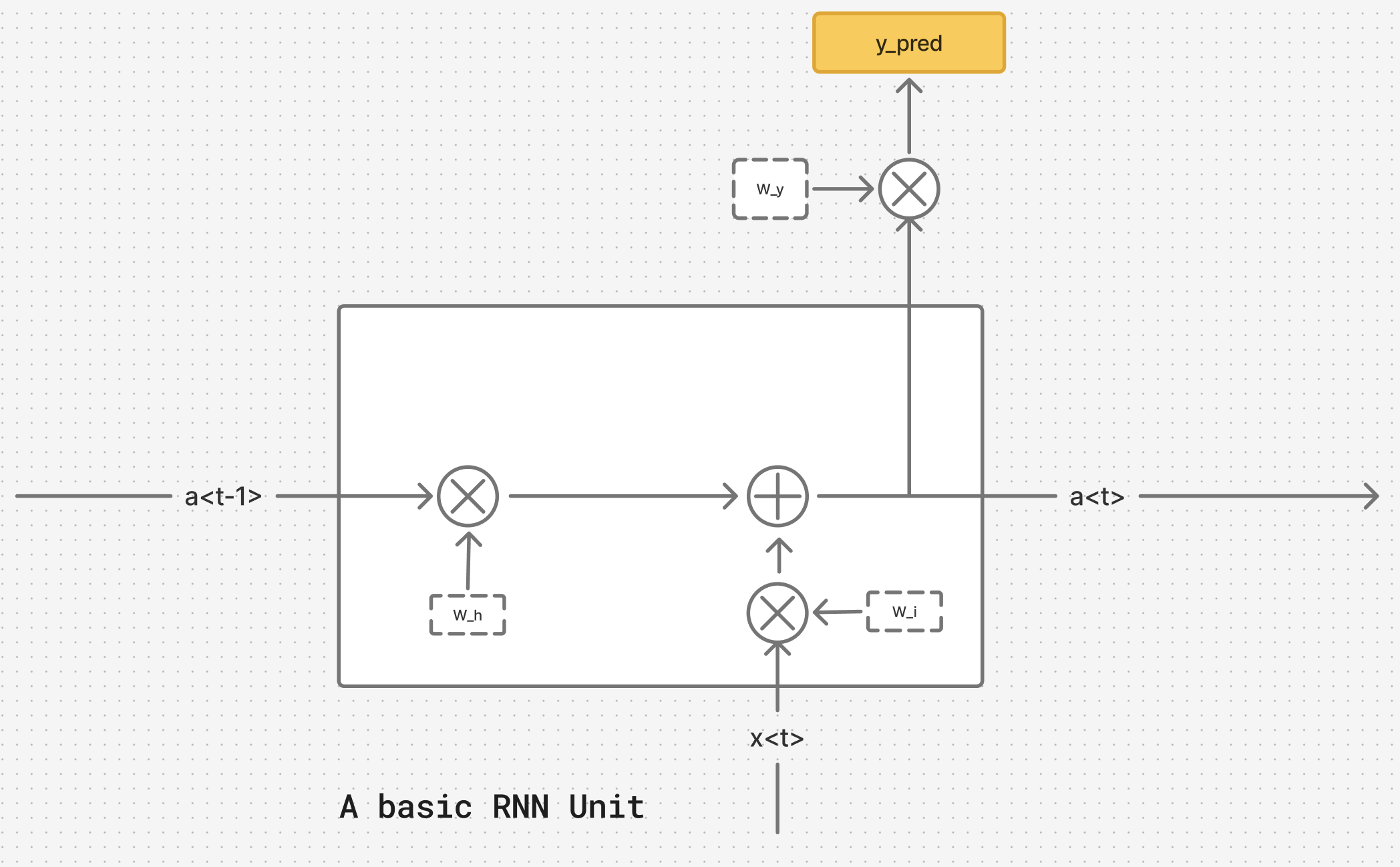
From the above diagram, we re-iterate the presence of two inputs for each unit: static & temporal. In this architecture, we are working on a training example where the entire sequence is already available, and there is no need to generate the next-in-sequence datapoint. As a result, $x^{<t>}$ is not dependent on previous unit $y^{<t-1>}$, as is in the case of sampling, where the output of previous unit $(t-1)$ is used as an input for the subsequent unit $(t)$.

Mathematical Interpretation

A. Forward Propagation

Assuming no of inputs $[T_x]$ = Assuming no of inputs $[T_y]$, we compute two components:

1. Hidden state value: $a^{<t>}$
2. Output unit: $\hat{y}^{<t>}$

For given parameters, $W_{aa}$, $W_{ax}$ & $b_a$ corresponding to Hidden state and $W_{ya}$ & $b_y$ corresponding to $\hat{y}$:

For every time-step 't':

$a^{<t>} = g[W_{aa} \cdot a^{<t-1>} + W_{ax} \cdot x^{<t>} + b_a]$

$y^{<t>} = g[W_{ya} \cdot a^{<t>} + b_y]$

We can further simplify equation (1) corresponding to $a^{<t>}$ by compressing two parameters $W_{aa}$ & $W_{ax}$ into $W_a$:

$W_a \sim [W_{aa} : W_{ax}]$

here the matrices $W_{aa}$ & $W_{ax}$ are stacked horizontally

If $\dim(W_{aa}) = (100, 100)$ & $\dim(W_{ax}) = (100, 10000)$, then

$\dim(W_a) = (100, (100+10000)) = (100, 10100)$

Using $W_a$ in $a^{<t>}$:

$a^{<t>} = g[W_a(a^{<t-1>}, x^{<t>}) + b_a]$

Now, $[a^{<t-1>}, x^{<t>}] \rightarrow p$

$p \sim \begin{bmatrix} a^{<t-1>} \\ x^{<t>} \end{bmatrix}$

here matrices $a^{<t-1>}$ & $x^{<t>}$ are vertically stacked

Finally:

$a^{<t>} = g[W_a \cdot p + b_a]$

B. Backpropagation Through Time

• Similar to ANN, the real learning happens in backpropagation, where we minimize the loss function by finding optimum values for the given parameters.
  • We use gradient descent to reach the optimal values
• To simplify the understanding, let us assume there is only one output for the network, that is present at timestep $T_x$.
  • The loss function as defined below depends only on one value of $\hat{y}$, instead of $\hat{y}$ at every time step

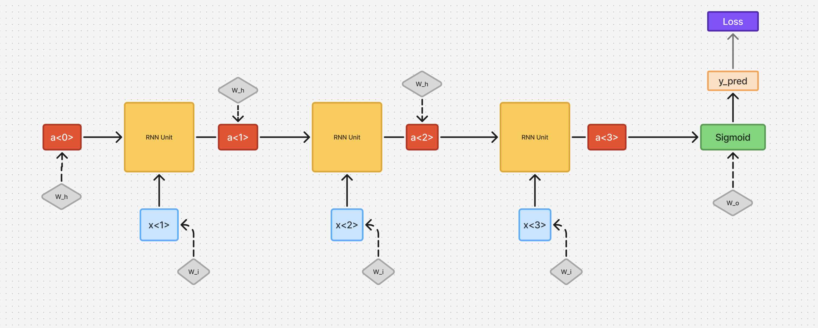
We use cross entropy loss:

$\mathcal{L}[\hat{y}, y] = -y \cdot \log(\hat{y}) - (1-y) \cdot \log(1-\hat{y})$

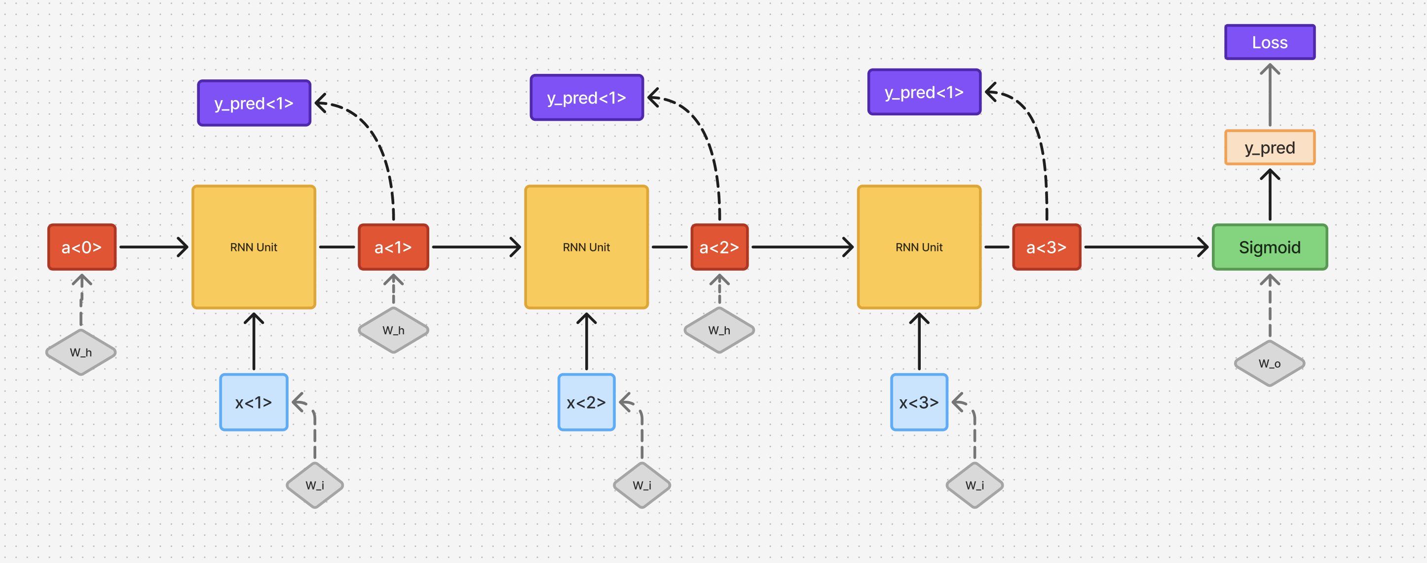
In case we predict an outcome at every timestep:

$\mathcal{L}[\hat{y}, y] = \sum \mathcal{L}^{<t>}[\hat{y}^{<t>}, y^{<t>}], \text{ where } t \rightarrow \text{timestep}$

Following are the parameters we will optimize:

• $W_{aa} \rightarrow W_h$: weights for hidden units
• $W_{ax} \rightarrow W_i$: weights for input units
• $W_{ya} \rightarrow W_o$: weights for output unit

Applying gradient descent for learning rate $\alpha$ :

$W_h = W_h - \alpha \cdot \frac{\partial \mathcal{L}}{\partial W_h}$

$W_i = W_i - \alpha \cdot \frac{\partial \mathcal{L}}{\partial W_i}$

$W_o = W_o - \alpha \cdot \frac{\partial \mathcal{L}}{\partial W_o}$

Our goal is to find $\frac{\partial \mathcal{L}}{\partial W_h}$, $\frac{\partial \mathcal{L}}{\partial W_i}$, $\frac{\partial \mathcal{L}}{\partial W_o}$ values to calculate optimal $W_h$, $W_i$, $W_o$

---

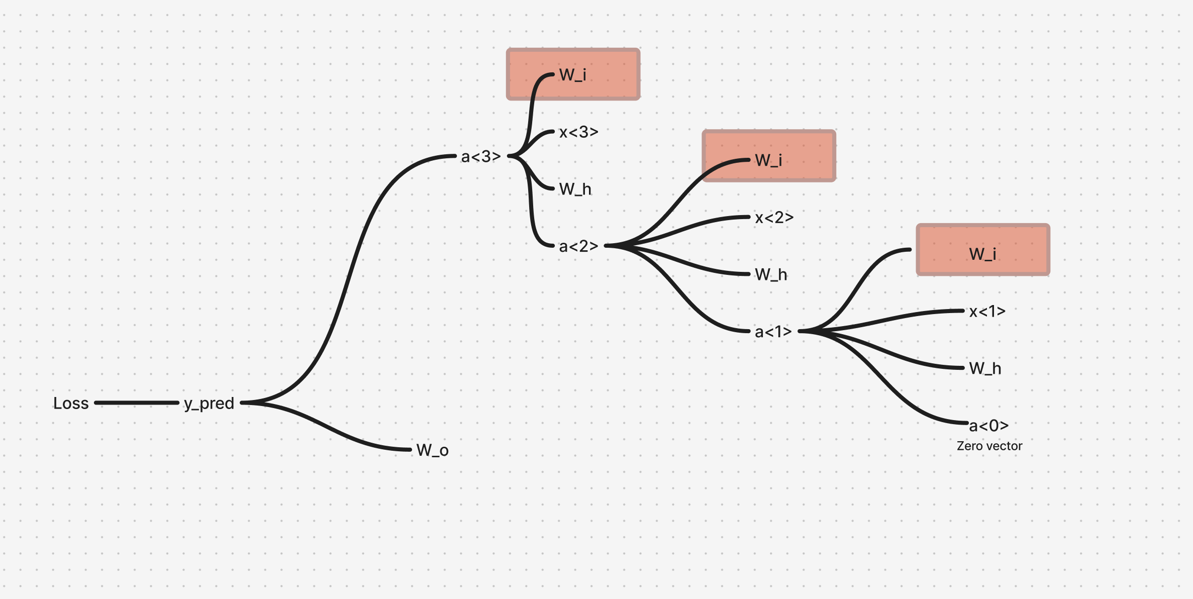
I. Calculating $W_o$

The given mind map shows the dependency mapping of functions, which helps to visualise the chain rule to calculate the gradient:

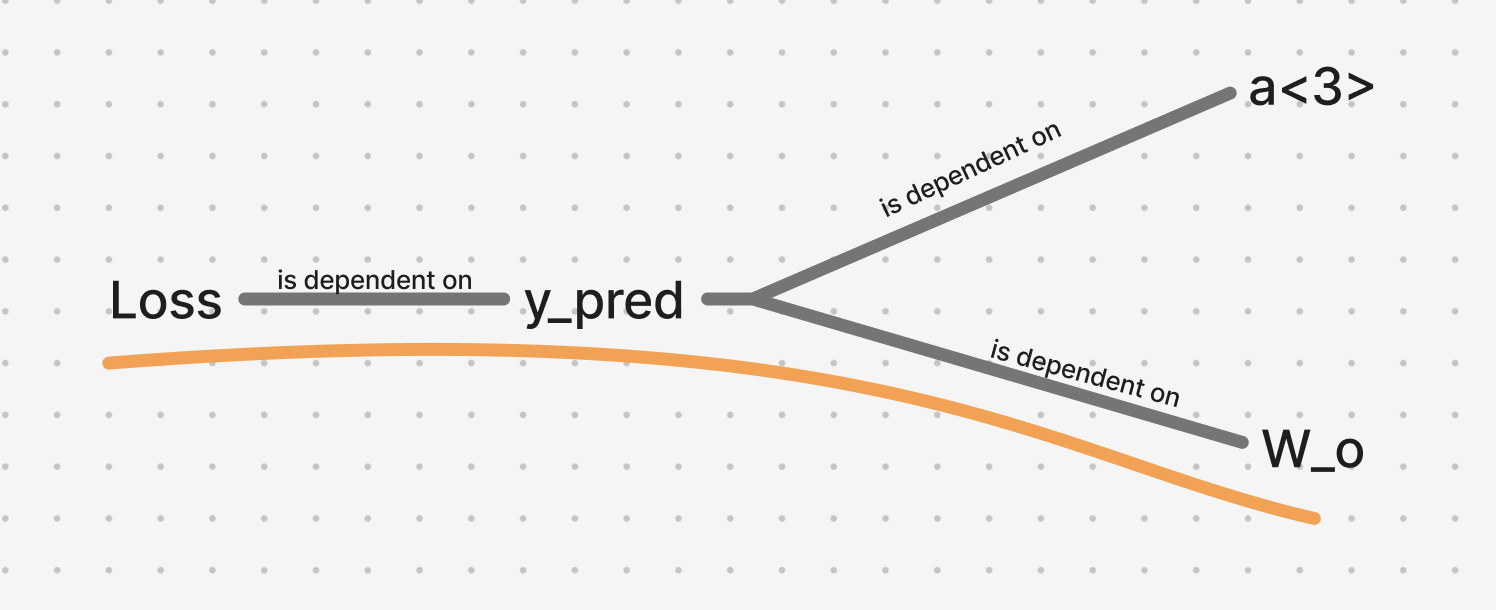From the above mapping we can calculate:

$\frac{\partial \mathcal{L}}{\partial W_o} = \frac{\partial \mathcal{L}}{\partial \hat{y}} \cdot \frac{\partial \hat{y}}{\partial W_o}$

using chain rule

---

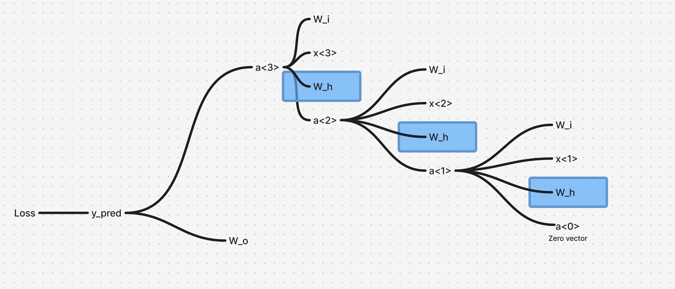
II. Calculating $\frac{\partial \mathcal{L}}{\partial W_i}$

From the above dependency mapping, we have 3 simultaneous dependencies that occur as we move back in timestep from $a^{<3>}$ to $a^{<1>}$, which can simply be added together, after calculating the gradient for each timestep.

For timestep 3:

$\left[\frac{\partial \mathcal{L}}{\partial W_i}\right]_3 = \frac{\partial \mathcal{L}}{\partial \hat{y}} \cdot \frac{\partial \hat{y}}{\partial a^{<3>}} \cdot \frac{\partial a^{<3>}}{\partial W_i}$

For timestep 2:

$\left[\frac{\partial \mathcal{L}}{\partial W_i}\right]_2 = \frac{\partial \mathcal{L}}{\partial \hat{y}} \cdot \frac{\partial \hat{y}}{\partial a^{<3>}} \cdot \frac{\partial a^{<3>}}{\partial a^{<2>}} \cdot \frac{\partial a^{<2>}}{\partial W_i}$

For timestep 1:

$\left[\frac{\partial \mathcal{L}}{\partial W_i}\right]_1 = \frac{\partial \mathcal{L}}{\partial \hat{y}} \cdot \frac{\partial \hat{y}}{\partial a^{<3>}} \cdot \frac{\partial a^{<3>}}{\partial a^{<2>}} \cdot \frac{\partial a^{<2>}}{\partial a^{<1>}} \cdot \frac{\partial a^{<1>}}{\partial W_i}$

Combining all three:

$\frac{\partial \mathcal{L}}{\partial W_i} = \left[\frac{\partial \mathcal{L}}{\partial W_i}\right]_3 + \left[\frac{\partial \mathcal{L}}{\partial W_i}\right]_2 + \left[\frac{\partial \mathcal{L}}{\partial W_i}\right]_1$

$\frac{\partial \mathcal{L}}{\partial W_i} = \frac{\partial \mathcal{L}}{\partial \hat{y}} \cdot \frac{\partial \hat{y}}{\partial a^{<3>}} \cdot \frac{\partial a^{<3>}}{\partial W_i} + \frac{\partial \mathcal{L}}{\partial \hat{y}} \cdot \frac{\partial \hat{y}}{\partial a^{<3>}} \cdot \frac{\partial a^{<3>}}{\partial a^{<2>}} \cdot \frac{\partial a^{<2>}}{\partial W_i} + \frac{\partial \mathcal{L}}{\partial \hat{y}} \cdot \frac{\partial \hat{y}}{\partial a^{<3>}} \cdot \frac{\partial a^{<3>}}{\partial a^{<2>}} \cdot \frac{\partial a^{<2>}}{\partial a^{<1>}} \cdot \frac{\partial a^{<1>}}{\partial W_i}$

Generalizing this for timesteps $T_x$:

$\frac{\partial \mathcal{L}}{\partial W_i} = \sum_{j=1}^{T_x} \frac{\partial \mathcal{L}}{\partial \hat{y}} \cdot \frac{\partial \hat{y}}{\partial a^{<j>}} \cdot \frac{\partial a^{<j>}}{\partial W_i}$

---

III. Calculating $\frac{\partial \mathcal{L}}{\partial W_h}$

Using the same dependency mapping from the previous calculation, we again have multiple simultaneous dependencies as we go down the timesteps.

Generalizing this for timesteps $T_x$:

$\frac{\partial \mathcal{L}}{\partial W_h} = \sum_{j=1}^{T_x} \frac{\partial \mathcal{L}}{\partial \hat{y}} \cdot \frac{\partial \hat{y}}{\partial a^{<j>}} \cdot \frac{\partial a^{<j>}}{\partial W_h}$

Drawbacks of Vanilla RNN

The major drawback of the RNN architecture is that it cannot work well on sequences with Long Range Dependency, as it suffers from the well-known Vanishing Gradient Problem.

Understanding Long Range Dependency

→ Sometimes in a language, sentences are framed in such a way that they have Long Range Dependencies, which means a word which comes earlier in a sentence influences what needs to come much later in that sentence.

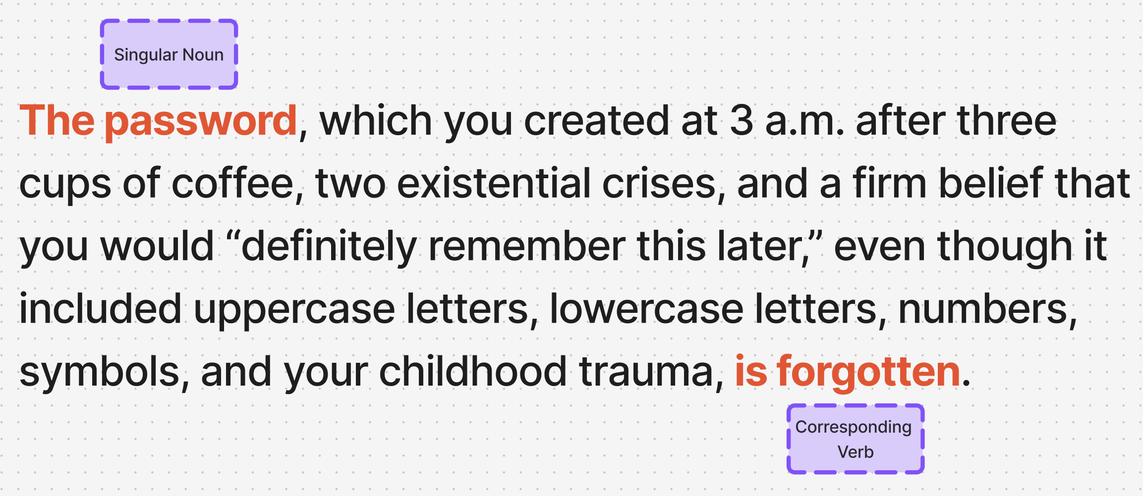
→ A Vanilla RNN architecture finds it difficult to memorize the context from earlier words onto words that come much later.

Why This Happens

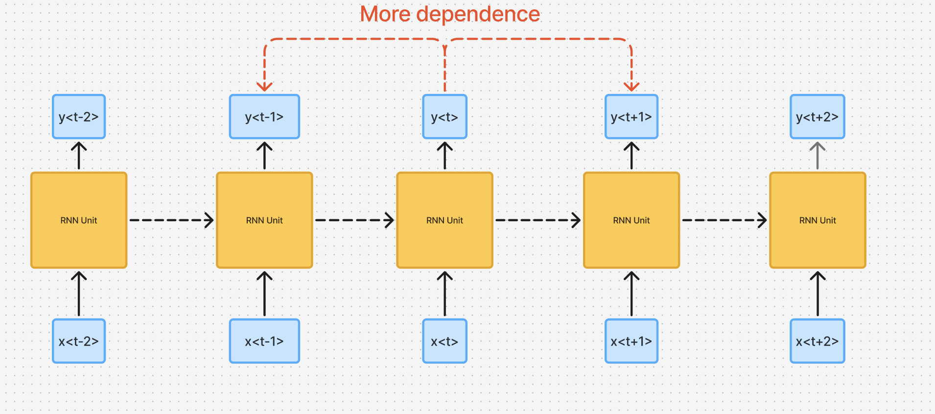
• This is because in this architecture, the output at a timestep $t$ is closely associated by neighbors of $t$ and not so much by distant neighbors

---

The vanishing gradient problem prevents vanilla RNNs from effectively learning dependencies that span many timesteps.

Therefore in order to capture the long range context, we introduce the concept of ‘Context Cell’ or ‘Memory Cell’ which acts as an additional input to these sequential units. This forms the basis of subsequent architectures in sequential modelling namely, Gated Recurrent Unit and Long Short Term Memory.